Monday, July 31, 2017

Kansas Water Towers as Seen by a Drone

As I headed home to Idaho last weekend, I made a few stops to test my new camera, an Apeman A60. The camera was slung beneath my Blade Chroma and setup to record video. I took screen shots of some of the video and would like to share them.

My first goal in shooting video was to show that flying around infrastructure is safe, as long as you keep a respectful distance and don't cross private property lines. Second, I wanted the video to show that drones are a safe and inexpensive way to inspect infrastructure. These still images could show more detail if it was used by a county or state employee who's job was to inspect infrastructure. Finally, a drone platform let's you see what the top of stuff looks like and gives a better feel for its placement in the community.

The Hays, Kansas water tower next to the Sternberg Museum. I made sure my drone did not cross the fence around the tower.
At 400 feet up, the water tower is way below the drone. Now we can see what's on top of the tower. This image is looking towards the East.
The Park, Kansas water tower. Again, I kept a respectful distance away from the tower.

Sunday, July 30, 2017

UAVSonde Data for NearSys Station, 30 July 2017

UAVSonde data were collected at 6:45 AM. Here are the data.

Altitude: 2,257 feet
Temperature: 78 *F
Relative Humidity: 39%
Pressure: 934.0 mb

Altitude: 2,663 feet
Temperature: 86 *F
Relative Humidity: 3%
Pressure: 917.6 mb

Tuesday, July 25, 2017

Manhattan Planet Walk

In 1999, I worked with the K-State Physics Club to create a Planet Walk for Manhattan, KS. While visiting family this summer, I took a quick trip out to the start of the Planet Walk to see what part of it still existed. In years past, I've discovered that parts of it were knocked over or removed. I was hoping I would find some parts of it were still standing when I visited this summer.

The Little Apple Planet Walk was set to a scale of one million miles per yard. This scale means the the sun is the size of a beach ball. It also means that the distance between the sun and Earth is 93 yards. A walk from the sun to Pluto was a walk of some two miles. That's a doable distance and one that can give you some pleasant exercise.

It was amazing how quickly one would walk between the sun the terrestrial planets of Mercury, Venus, Earth, and Mars. Then walkers would experience a large gap between Mars and Jupiter. The distance between the gas giants of Jupiter, Saturn, Uranus, and Neptune were equally large. Taking a Planet Walk is a good way to experience the vast and lonely distances that make up the outer solar system.

The Little Apple's Planet Walk begins at the entrance of the Linear Park Trail's entrance at Pecan Circle. This informative sign was created by Thomson Signs and donated to the planet walk  
Each planet's average distance from the sun was marked with a limestone pillar. The pillars were created by Manhattan Monuments and donated to the planet walk. Originally, each pillar held a stainless steel disk cut to the proper scale size of each planet. The KSU Physics Machine Shop made the disks.
Over time, walkers of the Manhattan Linear Trail removed the disks for each planet and knocked over the pillars. I know that Mercury's pillar is still standing, but those of the rest f the terrestrial planets do not. And I suspect the remaining planets aren't standing anymore either.

It was a fun project and I liked getting the donations that made it happen. I am especially happy that the Manhattan Parks and Rec went out of their way to get the walk installed. Thanks everyone for making its possible. I just wish people were more careful around it. I hope to get another one installed somewhere in the future.

Images Above Kansas State University

I made a quick flight above KSU (one of my old Alma Maters) with the Quadcopter and got two images worth keeping.

Looking toward the northwest from the southeast corner of the campus. Altitude is around 300 feet.

My quadcopter wasn't the only thing above KSU. Now I know what the campus looks like from a bird's perspective.

Thursday, July 20, 2017

Earth's Shadow

Many people have seen Earth's shadow, but were unaware of its presence. After the sun sets, or before it rises, there's about a 20 minute window to watch Earth's shadow projected on the atmosphere. It appears as a slightly darker blue band above the horizon with a reddish band above it.


I produced a short time-lapse movie of Earth's shadow in the west as the sun rises in the east. The movie has two parts. The first part is in visible light, or how we would see it with our eyes. The second part is through the eyes of near infrared. Interesting that the slightly smoky skies we're dealing with in the Treasure Valley prevents our eyes from seeing the anticrepuscular rays but that NIR cuts right through the haze. What are anticrepuscular rays? Well, crepuscular rays are the dark shadow of clouds projected into the atmosphere as lines or rays. Anticrepuscular rays are those cloud shadows projected onto the opposite end of the sky. They point to the anti-solar point, or the point in the sky are is opposite the sun.


You an see my Morning Movie at the NearSys YouTube channel.


Earth's shadow on visible light, or how your eyes would see it.


This is Earth's shadow in near infrared. Notice how much darker it appears.
 

Saturday, July 15, 2017

UAVSonde Data for NearSys Station, 15 July 2017

UAVSonde data were collected at 8:10 PM. Here are the data.

Altitude: 2,227 feet
Temperature: 103*F
Relative Humidity: NA
Pressure: 917.6 mb

Altitude: 2,811 feet
Temperature: 100*F
Relative Humidity: NA
Pressure: 914.6 mb

The GPS reciever misbehaved at high altitude. If this repeats, the GPS will be replaced.

Friday, July 14, 2017

Can Robotic Vision Guide a Robot Down a Row of an Orchard?

Based on this color-near infrared image, is this robot driving down the middle of the orchard row? Can the robot determine how much and in what direction it must adjust its driving path? Image from the NNU Robotics Vision Lab. 


Orchard work is labor intensive and labor costs money. In order to keep costs down, agriculture, along with manufacturing, is trying to automate processes. In agriculture, automated systems means things like programming robots to drive down the rows between trees in an orchard to inspect the fruit or spray the trees. For robot to drive through an orchard without crashing into trees, it must first recognize trees in its robotic vision, determine its location based on that image, and then plan a driving path. I was given an opportunity to analyze an image recorded by the camera system of a robot built by NNU and see what I could come up with. Here's what I did, using ImageJ to analyze the image above (as told by the images generated in each step). With a pinch of luck, this will help robots see trees from the orchard (forest).


First, crop the image. I took about the center 1/3rd of the image and it doesn't seem my method doesn't cares exactly how much of the image is cropped, as long as it includes the tree trunks.  


Next, split apart the three color channels and retain just the near infrared. Notice that the tree trunks appear very dark compared to the leaves, grass, and even the sky. On  cloudy day,  the sky should appear even brighter, which makes the next process even easier. 
The image is then segmented by setting a threshold using the Otsu method. However, in this case, I selected to invert the image by isolating the high end of the histogram. I suspect one could invert the image first and then let the Otsu method segment the image as it determined is best. Segmenting an image means finding a good threshold value in to which to split the image into either black or white pixels.  


After the image is segmented, its filtered to remove the more distant trees and grasses. The filtering that does this works by dividing the image into ten pixel groups and making every pixel in the group as bright as the brightest pixel in the group of ten. So it's called maximum filtering.  

Now the image is scaled. The scaling decreases the x-axis by a factor of 2 (scaling factor is 0.5) and the y-axis by a factor of four. So essentially, the image is being stretched vertically and shrunk horizontally. The image is shrunk in the x-axis to keep the image size from becoming too large. 


After scaling, the image is cropped to keep just the middle third. The stretching and cropping is repeated a second time.  
This is what the image looks like after the second round of scaling and cropping.


Now the image is made into a binary file. In other words, each pixel is just a 1 or a 0.
In this step, the image is skeletonized. That means the middle of each region is replaced with a line running through its middle. So notice that this process has turned the tree trunks visible in the near infrared image into a series of vertical black lines. 
Now the robot's vision system just needs to detect the black lines across the image. I think the reference line can be taken at any height across the image.
Final Thoughts
My feeling is that the vision system should count the x-axis location of a black line as it goes across the image. Since the lines are a single pixel wide, the location of each black line becomes a single number. The location of each black pixel must be taken in reference to the center of the image (in other words, the origin of the horizontal sampling line is the center of the image. Pixel locations left of the center of the image have negative values and pixel locations right of the center of the image have positive values. Now add the pixel values together. The sum indicates the center of the tree rows relative to the center of the image. If the sum is positive, then the robot needs to drive forward and right. If the sum of the pixel values is negative, the robot needs to drive forward and to the left. And of course, if the sum is zero, the robot just needs to drive forwards. The absolute value of the pixel sum indicates just how far off the center the robot is.


For higher accuracy and certainty, the robotic vision system might want to take measurements across the final skeletonized image in several rows.

Imaging Fruit from the Ground Up

A suggestion given at a program review in the Robotics Vision lab where I'm working this summer was to image fruit from below the trees. The reasoning is that the fruits would hang down where the leaves can't block the view to them. It sounds like a good idea, however, I found the thermal imager would respond well to this. Why?


Yep, there's fruit here. The peaches are still green, but visible from beneath the tree.
The thermal infrared image from near the center of the visible image above. There are peaches to the left and bottom left of the dark hole above the center of the image.
The issue with the Seek Reveal (at least with the way I have it set up) is that it scales the colors of its image based on the range of temperatures it detects. Looking up means the imager will see the sky. Now the sky is very cold in thermal infrared, meaning the sky becomes the black color setting. The warmest tree leaf or fruit meanwhile become the white color setting. Since there is such a large difference between the cold sky and the warm leaves and fruit, any difference in temperature between a fruit and a leaf is tiny in comparison. Therefore, no difference between fruit and leaves can be made out in the image.


Thermal imaging may still be useful for distinguishing between fruit and leaves with robotic vision. That's because fruit, being more massive than a leaf, should maintain a warmer temperature after a cool night. However, for thermal imaging to detect this, the thermal image needs to be taken without the sky being in view. Or, the thermal imager can't auto-scale its image based on temperature extremes it detects.


I may need a different thermal imager to make robotic vision possible.    

Wednesday, July 12, 2017

ImageJ

Jim, a friend reading my blog, suggest I try out ImageJ for image processing. I had never heard of this program before and needed a few days before I could find the time to check it out. And boy am I glad I did.


ImageJ is a Java app that was developed by the National Institute of Health (the project developer was Wayne Rasband) to perform image processing. You can download the application from its location on the NIH Website.


After installing it n my laptop at NNU, I just click the ij executable file to get ImageJ's simple to use menu to pop up.


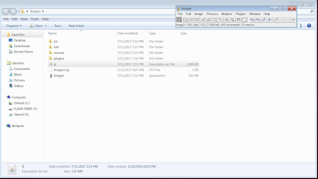
That's right, the ImageJ window is pretty small. Just a simple menu, really. 


It just took six total clicks to split a color image into its three channels. First, I had to open the image with File, Open, and then click on the image I wanted. After opening the image, I then used 3 more clicks to split the color image into its three RGB channels. I clicked on Image, Color, and Split Channels. The original color disappeared and was replaced with three images, one for each color.


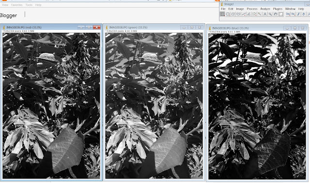
I like that ImageJ automatically gives each image window a name that includes its color layer. 
Next I tested the subtraction of images. Subtracting images can be important for isolating cherries in an image of a cherry tree, because green leaves are bright in both red and green but cherries are only bright in red. Subtracting images requires the use of the Paste Control application. You'll find it under the Edit option.


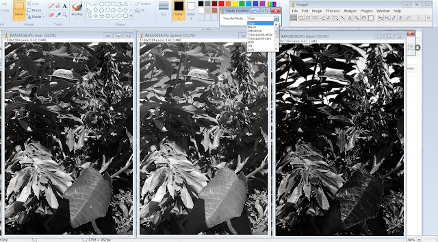
The Paste Control Application showing some of its paste options in a pull down menu.
One color layer is subtracted from a second one first making sure that the Subtract option in Paste Control is selected. Then click on the color layer to be subtracted and then clicking Edit and Copy in ImageJ. Then click the second color layer, the one you want to subtract the first layer from, and then click Edit and Paste. Note that the order of the subtraction is important. Subtracting the red layer from the green layer does not produce the same result as subtracting the green layer from the red layer.


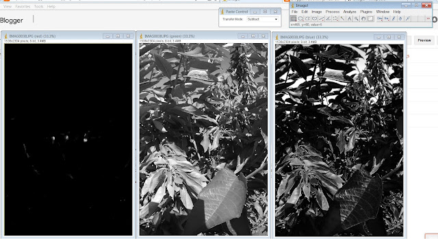
The red color was on the left, but it's been converted in the red layer minus the green layer with just a few clicks. 
An image can be segmented with ImageJ by first finding a global threshold. Setting a threshold is an interactive process, in that you can shift two sliders to set the high and low limits, if you desire. You can also let ImageJ set the boundaries. So click Image, Adjust, Threshold. The Threshold application opens up and the clicked layer suddenly appears as a segmented image with the default threshold values.


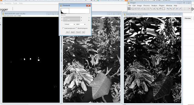
The Threshold application pops up in its default setting. Notice the modified red layer is displayed in the current threshold value.
You can now adjust the sliders in the Threshold application to set what range of pixel values to threshold with. It's interactive, so as you adjust the left and right limits, the image displays what it will look like under that threshold setting.


After applying a threshold and segmenting a layer, you can detect the edges of the image by clicking Process and then Find Edges.


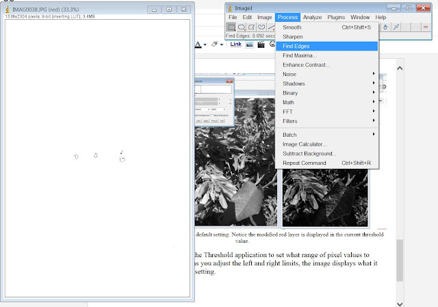
These are the edges of the segmented layer displayed above.
Images, or layers, can be merged together to create a new color image. This is accomplished by clicking Image, Color, Merge Channels... Under the Merge Channels application, select which image to make which color and then click Okay.


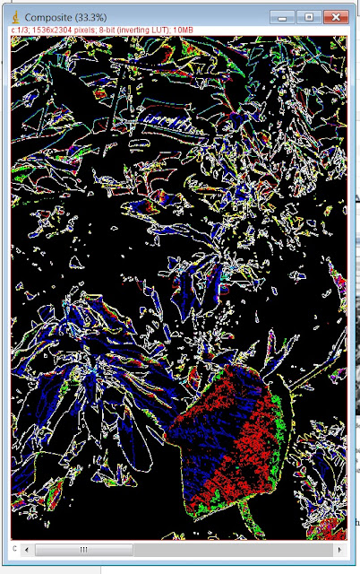
A three color image of the edges detected in the original color image. I don't know if this is particularly useful, but it is pretty cool looking.
Counting the number of objects in an image is more important than creating pretty images of edges. So that's what I'm working on next. More about that soon (I hope).

Monday, July 10, 2017

UAVSonde Measurements of Surface and Air Temperature Multiople Times Throughout the Day

I fly my UAVSonde flights once per week, usually on the weekend, to gather temperature, pressure, and relative humidity once a day. I began to wonder how these conditions changed throughout the day. I know the ground temperature increases until around 4:00 PM before it begins falling again. But does this hold true 400 feet above the ground? I am investigating conditions at an altitude of 400 feet because that's how high my drone can legally fly.


So I ran the same sensors and collected data the same way five times on Sunday, July 9th. Now it was stinking hot on Sunday. My part of Idaho broke a temperature record with highs above 100 degrees. Also, the quadcopter lifted off from my driveway. That driveway was extra toasty. It was obviously the case if you looked at the driveway and the neighboring lawn with the thermal imager. Anyway, once I completed  the first flight, I was committed to repeating the rest of the flights in the same manner. Below are the results I got from the flights. The time is in 24 hour time.


First notes,  GPS receivers have errors in their measurements, so I needed to take an average ground elevation and air altitude for these charts. Second, the pressure sensor may be effected by the temperature. Third, the surface temperature is taken right above the cement driveway.


The first chart shows that the ground temperature did indeed increase throughout the day and began cooling at around 3:00 PM. It then spiked in temperature later in the evening. The air temperature at 400 feet AGL lagged behind the surface temperature by 7 to 10 degrees before cooling off by 7:00 PM.


The second chart shows the air pressure at 400 feet AGL is always lower than the surface pressure, but that amount of difference changes throughout the day. Also that the surface pressure spiked at around 7:00 PM. Meanwhile, the air pressure at 400 feet AGL spiked earlier at around 2:30 PM.


I really need to repeat this experiment again when it's not quite so hot. I'll also experiment with calibrating the pressure sensor with temperature in order to remove this possible effect. Finally, I'll launch the quadcopter from the lawn.


It's said you can look up lots of information on the Internet these days. It's probably true that someone already knows how the temperature of the air several hundred feet above the ground changes throughout the day. But I say why look it up when you could find out for your self. In the process, you learn more STEM and the importance of measurement. And you'll develop more skills and hone the ones you already have. An that's not a bad way to spend a Sunday afternoon.  

Flame Wheel Quadcopter

Part of my summer research is trying to find a good drone for my Introduction to Engineering class next year. I feel this list of requirements is suitable for this task.


The drone is affordable
The drone is student-built (this way students get a better idea of how it works)
The drone is flexible in its control system
The drone can carry a payload


Dr. Bulanaon suggested I look into the DJI Flame Wheel as a class drone. So we ordered one and I began assembling it after it arrived. The Flame Wheel was the second drone I had seen, so it was nice to have a change to work with it.


Open the box and you'll find bags of drone parts.
I needed to download the directions before I could begin assembling the Flame Wheel.  I also needed to watch a video to fill in the assembly steps not covered in the online directions. But after a couple of hours or assembly, disassembly, and reassembly, I ended up with this fine product.


Assembled and looking for an RC receiver.


The Flame Wheel is a generic drone, it's designed for any number of RC systems and batteries. So after a little more investigation, I've developed the following shopping list.


FrSky RX8R 8/16 channel, S Bus receiver
FrSky Taranis Q X7 16 channel, 2.4 GHz ACCST transmitter
Storm 3s 5,500 mAh LiPo (with XT60 connector)


The 16 channel RC control system will allow remote pilots to control the flight of their drone and the gimbal carrying the drone's imagining system. However, there will be an extensive setup procedure to unite the RC control system to the flight controller (NAZA Lite) used by the Flame Wheel. I'll update my blog with the procedure I went through, so keep your eyes opened.


The drone will be Bind-n-Fly, meaning the receiver will only respond to commands from the transmitter its bound to. This way, many students can fly their drones simultaneously without interfering with each other. Of course, with multiple drones airborne, students will need to work in teams of pilots and visual observers for safety. Otherwise, I think my students are really going to like the Flame Wheel. I know their teacher is.


Sunday, July 9, 2017

Sunspot AR2665

I read this morning in my email from Space Weather that the sun was rotating a new sunspot towards Earth. After my success with photographing Daphnia through a microscope, I decided to attempt the same thing with my 90 mm cataoptric.

The sun magnified 20 power as seen through a cellphone camera. The sun is bright enough with even the solar filter that a less than steady hand could get this image.


Sunspot AR2665 is nearly the size of Jupiter, which is 11 times larger than Earth. The sunspot has produced an M-class solar flare and a radio blackout over Australia and Asia. We might see coronal mass ejections from this sunspot, which increases our chances of seeing aurora. Keep your eyes and ears open.

UAVSonde Data for NearSys Station, 9 July 2017

UAVSonde data were collected at 7:30 AM. Here are the data.

Altitude: 2,240 feet
Temperature: 100 *F
Relative Humidity: NA
Pressure: 916.4 mb

Altitude: 2,680 feet
Temperature: 93 *F
Relative Humidity: NA
Pressure: 914.6 mb

The UAV launches from the cement drive way, so the ground temperature is higher than expected.

Thursday, July 6, 2017

Using Octave in Place of Matlab

Matlab, from MathWorks is a very powerful program designed to perform technical computing with matrix-based mathematics (which includes arrays). It's used extensively by mathematicians, scientists, and engineers to analyze their data. I'm using now at NNU to analyze images of fruit trees recorded by drones and from the ground.


Checking the MathWorks website, I see there's a home edition available for $149. Additional Add-ons at $45 each allow you to increase the functionality of Matlab and even perform simulations (using Simulink).  The home edition webpage contains links on how Matlab was used for things like an Arduino-based weather station. And at $145, the cost really isn't too much when you consider how much we pay for other productivity software.


I'm however, looking into using a program named Octave to perform the same analysis that I am using Matlab do to. The reason I'm testing Octave is that it's freeware under the GNU General Public License. Using Octave in place of Matlab let's my classroom analyze drone-recorded images while saving money. My students will  then be able to install the freeware at home and complete their homework at their leisure (and I hope take up an interest in mathematical computing).


You can download the Window's version of Octave  and then install it on as may PCs or laptops as needed. I found that Octave, like Matlab does not have an image package built in. So you'll also need to download the Image Package separately and then install it. Loading the Image Package is done from the Octave Command Window by typing the following command,


pkg load image-2.6.1.tar.gz


Note that every add-on package is installed using the same syntax. In the case above, the Image Package is a compressed file called image and its version number is 2.6.1. The only issue I'm less than happy about how Octave doesn't generate a message after the successful completion of a package install. So I was uncertain if the install was complete or of I needed to wait a while longer. However, Octave will generate an error message if the install fails.


You might want to install multiple packages into Octave, so repeat the above command with every package. If you lose track of the installed packages, type the command below into the Command Window.


pkg list  


Octave generates a message listing every package installed as shown below.


After installation, you'll need to load the Image Package every time you start Octave. This is done in the Command Window by typing the following command,


pkg load image


Well, that's all you need to do to install Octave and its Image Package on a PC or laptop. I'll keep testing Octave to verify it does everything my classroom needs to analyze images from their drones next year. The 2017-2018 school year promises to be very exciting and I think my engineering students are going to love it.


Tuesday, July 4, 2017

Photopolarimeter Data for July 3rd

I decided to give the photopolarimeter another test this week, now that we're experiencing summer weather. It's the same instrument I used for February 12th's blog entry http://nearsys.blogspot.com/2017/02/a-modification-to-balloonsat-recording.html?m=1, but modified to see if it could also detect polarization in blue or violet light.

To reach the shorter wavelengths, I taped a second polarizing filter to the first. I was hoping the two filters would act like a single filter with more narrowly spaced lines of polarization. It appears that this did help bring out polarization differences in the blue, but not violet to ultraviolet.

Here are the results for your pleasure. As you'll see, I need to do some more measurements to see if my results from the 3rd are typical.

Sunlight intensity peaked between 3:00 and 4:00 PM for most light wavelengths. And you notice the effects the cloud had between 4:00 and 5:00 PM. However, it appears blue and violet/ultraviolet didn't get the message. They increased in intensity all the way to between 6:30 and 8:00 PM. 
The colors of the sky were brighter in the East-West direction from 12:30 to 4:30 PM and then brighter in the North-South direction from 5:00 to 8:00 PM. But unlike blue, their total intensity's did decrease after 3:30 PM.

The violet/ultraviolet wavelengths were an anomaly. The sky continued to get brighter in this portion of the spectrum until 6:30 PM. The clouds also had a smaller effect on the sky brightness in this region. Odd.


Monday, July 3, 2017

Paper Chromatagraphy

I need to prepare a paper chromatagraphy lab for Advanced Placement Chemistry. The subject is a lab that lots of high school chemistry students have performed, but it sounds like AP students could use a refresher. Besides, it gives me a lab that these advanced students can do their first day back to school without over racing them. It doesn't hurt that the AP test asked a question on this topic. So here is the results of the first paper chromatagraphy lab I've done privately for myself at home.

First, find a colorful leaf to extract the pigments from. I choose a plant that had strong red pigmentation this spring.

A leaf from my front yard. This use to be more redder this spring.

Before performing chromotagraphy, the sample's pigments must be extracted. This procedure was the first experiment I performed for this lab. So two popular solvents are water (the universal solvent) and propanol and I tested both for this experiment.

The solvents can't do their job unless the pigments inside the leaf are not exposed to the solvents. Therefore I cut two leaves per solvent into thin slices. Then I added them to small glass bowls filled with their designated solvent.

Sliced leaves in water on the left and in 91% isopropanol on the right. Barely cover the leaves in solvent (unlike what I initially did) or else the concentration of pigment will be too small.

The solvents were hot, I microwaved the water and soaked the glass bowl of alcohol in a hot water bath (I have a bad feeling about what would happen if I were to microwave alchol). After soaking the leaves for over 30 minutes, place chromatagraphy strips into each glass container. For my strips, I used strips of a coffee filter my wife was unhappy with.

You'll notice that the alcohol was more effective at pulling pigment out of the leaves. Does this mean the green pigment (chlorophyll) is not polar?

There are intermolecular forces that pull solvent up the chromatagraphy strip. It's strongest for water since it rose to the height of the strip much faster than the alcohol. In this case, the intermolecular force was probably hydrogen bonding between water and cellose.

After the water was finishing climbing up and soaking the coffee filter chromatagraphy strips, I removed them and made some measurements.

The water-solvent strip is on the left and the alcohol-solvent strip is on the right. It's easy to see the pigment when extracted by alcohol. The pigment was not extracted by hot water.

Just extracting the pigment is not enough. The pigment's R-factor, or retention factor must be measured. It's calculated by dividing the length the pigment travelled by the length the solvent traveled, or the solvent front. My measurement of the alcohol strip was as follows.

Solvent Front: 1.50 inches
Pigment Line: 1.15 inches
R-factor: 0.77

What's Next?
So first off, I didn't extract enough pigment. I need a more concentrated solution of pigment and a larger quantity. Using more leaves, less solvent, and crushing the leaves should be effective in this regard. Greater pigment concentration means the pigment line will be darker and Amy pigments of lower concentration will become visible.

Second, I want to see how far water will draw up the year's pigment. Therefore, I will need to extract the pigment with alcohol and place a drop on the chromotagraphy strip. Then place the strip in a water solvent. A comparison of R-factor in water and alcohol should indicate the degree of polarization in the pigment molecule.

I'll let you know what happens next time.


Sunday, July 2, 2017

UAVSonde Data for NearSys Station, 2 July 2017

UAVSonde data were collected at 7:20 AM. Here are the data.

Altitude: 2,240 feet
Temperature: 89 *F
Relative Humidity: NA
Pressure: 918.4 mb

Altitude: 2,676 feet
Temperature: 78 *F
Relative Humidity: NA
Pressure: 914.6 mb