Friday, June 30, 2017

Daphnias or Water Fleas

Earlier this week I attended a workshop for teachers selected for Partner in Science grants by the M. J. Murdock Charitable Foundation of Vancouver, WA. At the workshop, I learned more about designing inquiry lessons and labs for science.

One of the projects we teachers completed was a lab to measure the heart rate of Daphnia. These crustaceans live in fresh water and about a millimeter across. As a result of their size, a microscope is needed to study them. We use stereomicroscopes and a magnification of ten power. The microscope allowed us to see the internal organs of the Daphnia. So as you can image, it was pretty cool. So cool in fact that I brought the camera lens of my cell phone up to the eyepiece to record an image. U needed to back off the lens slightly from the eyepiece and was able to capture images like the one below.

Daphnia have one eye and it's the dark spot on the upper right. Feeding arms which are spiky appendages are located to the right of the eye.

Since the still images were as successful as they were, I attempted to record a video next. The problem here was that I couldn't hold the cell phone still enough. Perhaps a small tripod is in order here. Nevertheless, the video did have an acceptable level of success.


My image and video demonstrates that students can successfully record microscope data with their cell phones. It's not always the best quality, but it's good enough to make cell phones an easily accessible science tool. By editing their images and video, students can create very informative graphics. Here's to the cell phone in the science lab. Just don't spend all your time texting.

June Weather for NearSys Station

The temperature for June increased roughly 15 degrees Fahrenheit. The gaps in the data are due to travel days, a risk that teachers experience during the summer months.


There was no snow in June (as expected) and 0.06 inches of rain. As a result, it's now very important the lawn at NearSys Station get watered daily (it's a desert here).


Segmenting Cherry Tree Images

It's difficult to segment images of fruits and fruit trees when their colors are very similar. Last week the public could pick their own cherries at fruit orchards like Williamson's (we got 20 pounds). So I took the opportunity to record visible, near infrared, and thermal infrared images of some of the cherry trees prior to picking fruit. Then today I tried my hand at segmenting the images.


The image I started segmenting
First my script separated the three color layers of the images. Then it compared the three layers so I could see how different they were. I discovered that the red leaves have a lot of red in them (very surprising).


Red layer on the left and green layer on the right. Notice that the leaves are only slightly darker in red than in green. On the other hand, the red cherries are too dark to appear in the green layer.
To create an image that Matlab could work with, I subtracted the green layer from the red layer to create a new image. Notice how well the cherries stand out from the leaves now.
Only cherries and a few stems/branches show up now. 
The resulting cherry layer could be segmented after determining a threshold value of intensity. The final results are displayed below.


From left to right: The original image, the separated cherries, and the segmented cherries.
Three obvious cherries appear in the final segmented image. The smaller dot is a cherry partially exposed behind a leaf. What does not show up are the cherries in the shadows of leaves. I want to experiment with bringing them out. Then I'll be ready to start measuring the size of the segmented regions and count them. Perhaps I'll even look into converting the blobs into elliptical circles for better assessment.


Happy Asteroid Day

June 30th is Asteroid Day. Why? Because on in the morning of June 30, 1908, a large meteor or comet impacted near the Tunguska River in Siberia. The first person to make a systematic investigation of the event was Leonid Kulki in 1927. What he found was unlike anything that anyone else had ever seen before in history.

Trees where knocked over in a pattern radiating from the center of the blast zone. Some 80 million trees over an 800 square mile region were damaged or destroyed.

It wasn't until 1945 that humanity witnessed another scene like this in the atomic bomb blasts in Japan.

Calculations indicate that the meteoric body responsible for the blast witnessed in Tunguska exploded with the force of around 4 megatons of TNT. That's the force found in a sizable hydrogen bomb. occurred over a city, the city and its population would have been destroyed.

Impacts like this are bound to happen again. In fact, it may be one 66 million years ago that's responsible for our rise. The reason dinosaurs are the top species today is that they didn't have a space program. We have one and need to be doing more with it to protect ourselves from extinction.

An event like this could be the end of humanity. Image from the BBC.
 Asteroids are more likely to be a source of resources and wealth than destruction, if humanity takes positive action. Organizations like the B612 Foundation are trying to prevent the worst aspects of asteroids while organizations like Planetary Resources is trying to take advantages of the best side of asteroids. Asteroid mining is going to take a coimbinationation of robotics and astronautics. So I encourage every school to add these topics to their curriculum. Who knows, you could be saving Earth or making a future trillionaire.  

There are over one million millionaires today and over 1,000 billionairs. But the are no trillionaires yet. I bet this is how we get the world's first trillionaire.

Saturday, June 24, 2017

UAVSonde Data for NearSys Station, 24 June 2017

After a three week delay for repairs, UAVSonde data were collected at 6:30 AM. Here are the data.

Altitude: 2,263 feet
Temperature: 57 *F
Relative Humidity: 48%
Pressure: 918.4 mb

Altitude: 2,572 feet
Temperature: 68 *F
Relative Humidity: 14%
Pressure: 917.6 mb

There's evidence for a temperature inversion over NearSys Station. The fact there was no surface winds fits with that pattern.

Friday, June 23, 2017

Finding the Edges of Segmented Images and then Stacking them Together

I've now segmented the separate colors on a thermal image and found its edges. Let me explain what I mean in today's blog entry

Segmenting is where Matlab determines whether or not a pixel value is high enough to meet a threshold. If it is, then the pixel is changed to white. If not, then the pixel is changed to black (there is no pixel values in between). The result is a stark black and white image. There are many ways to set the threshold. Aside from arbitrarily setting  the threshold, Matlab can evaluate the intensity of the pixels in an image and their frequency, or often a pixel of that given intensity appears in the image. A graph of the frequency and intensity of pixels is called a histogram and looks like this.

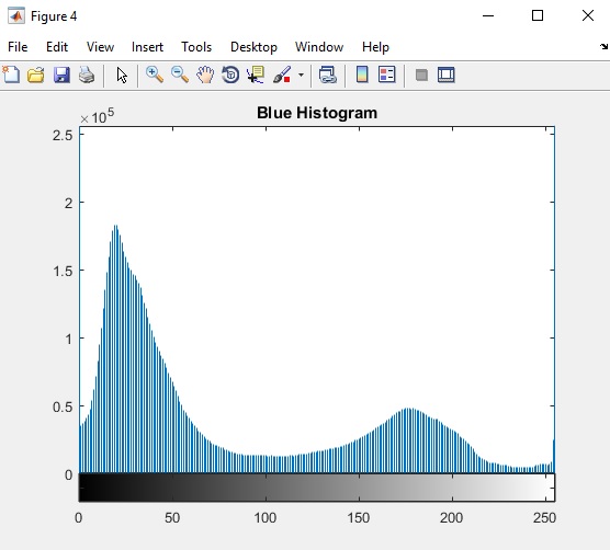
Histogram of pixel intensity in the blue layer of an image. The horizontal axis is all the possible intensities of pixels (since this histogram came from an eight-bit image, the largest possible intensity is 255). and the vertical axis is the number of pixels in the image with that intensity (note that the number is in 10,000). 

A possible good pixel intensity value to use in segmenting the blue layer of this image is 100 because it forms a nice valley in the histogram. Using a threshold of 100 means the pixels responsible for the peak around 35 would appear black and the pixels responsible for the peak around 175 would appear white.

Matlab can go do better at picking a threshold that we can looking at a histogram. By calculating means and variances (standard deviations squared) of pixel values, Matlab can determine an optimal threshold level for an image layer. The method is called Otsu's Method and it finds a threshold that minimizes the variances within a segmented region and maximizes the variances between the segmented regions. In other words, it splits an image into regions where the the pixels within each black regions are as close together in intensity as possible and the pixels in a white regions are as close together in intensity as possible. At the same time, the intensity of pixels between the black regions and the white regions are as far apart as possible. You can see this is making the segmented image as stark in contrast as possible.          

The Matlab command to find this magic threshold value looks like this.

[T, SM] = graythresh(image)

The input to this command is a two-dimensional array (a single color of an image) called image and the outputs are the optimal threshold value (T) and the separability measure (SM). Really, all one needs to segment an image after this command is the threshold value. Threshold (T) is a floating point number between 0 and 1. As a side note, SM is also a floating point number between 0 and 1 and the higher the value of SM, the better an image can be segmented.

Once the threshold value is known, the image is segmented using the following Matlab command.

segmentedImage = im2bw(image, threshold)

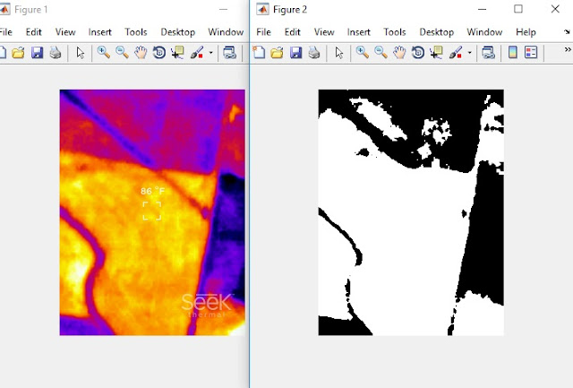
On the left is the original thermal image taken during descent above Gypsum Creek near Newton, KS. On the right side is the segmented red layer extracted from this image. 
In edge finding, Matlab looks for strong change in the intensities of two neighboring pixels. If the change in intensity is above a threshold level, then a black pixel (pixel intensity of zero) is drawn at the location of the pixels. There are many options available to the EDGE command detect edges. The most powerful method is the Canny Method and its Matlab command looks like this.

[edgedImage, threshold] = edge(image, 'canny', T, sigma)

The array edgedImage is the output of this command.
threshold is a vector (two dimensional array) that the Canny method uses to determine edges. It is not required and the EDGE command will calculate the value.  
image is the input image.
'canny' is the method the EDGE command is to use
T is a threshold value passed to the EDGE command to use to find edges. This variable can be left blank and the EDGE command will determine the appropriate value. If left blank, the variable T will be set to threshold at the end of the calculation.

So when I ran this command, I set its values as follows.

[canny1, T1] = edge(imageLayer, 'canny', [ ], 1);   

This may not be very useful in everyday images as you can see below.

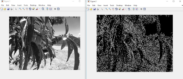
On the left is the red layer of a color image of a fruit tree. On the left is an image of the edges found in this picture. Because of the curves in the image and the subtle changes in pixel intensity, the edges found are a series of dots. 
But when a image is segmented first, the detected edges look more meaningful as shown below.

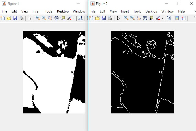
The left image is the segmented red layer of the thermal picture.  The right image is the edges detected in the segmented red layer. 
Recall that the color layers of an image is just a two-dimensional array. Well, Matlab can add those arrays  together to create a single image as if they were stacked together. Where two white pixels overlap each other in the stacked layers, the sum of the pixels remains 255 (a byte can't hold a value greater than 255). Where two black pixels overlap each other, the sum of the pixels is 0. Where a black pixel overlaps a white pixel, the sum of the pixels is 255. It's apparent that stacking black and white images together through array addition creates a new image of the sums of the edges of each image being stacked. Below is an example.

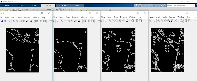
From left to right, the images are edges in the red layer, edges in the green layer, edges in the blue layer, and the stacked image of all three layers.
To make the stacked look more like we expect to see, I inverted the colors.

        
Finally, I created colored images from each layer and then concatenated them together. This turned out more difficult than I expected because each color's edge image is an array of logical values. In other words, each element in the arrays was either a 1 or  0. This creates two problems. First, the brightness of a pixel of value 0 or 1 are both very black (or close enough to black). Second, you can't concatenate three arrays of logical values. So the first step was to convert the logical array into an integer 8 array (so an array element, or pixel) could have a value of 255. I did this with the following command.

doubleRed = uint8(edgeSegmentedRed);

Then I multiplied each element in the integer 8 array by 255. This left the black pixels at zero and the colored pixel at 255. That command looks like this.

red255 = 255 * doubleRed;

After completing these steps for all three layers, I could concatenate them together with this command.

NewColor = cat(3,red255, green255, blue255); %restack or concateneate the images

It's important the order of the stacking be correct or else the product is an image where the individual layers are not shown in their proper color. when completed, the concatenation created the following picture.
The resulting image from edged segmented layers.
 Not too bad for a days work. what it all means I don't know yet. But I'll figure something out eventually.


Thursday, June 22, 2017

Separating Color Layers in a Digital Image

I'm learning to use Matlab to do image analysis this summer at Northwest Nazarene University (Nampa, ID). The task before me is to learn how to use images taken from drones to count the number of blooms or fruits on a tree. All digital images are three dimensional arrays. The first two dimensions are easy to understand, they're the height and width of the image. The third dimension is color and there are three layers there. So a digital image might be a 2,000 by 3,000 by 3 array. And arrays are an easy mathematical structure to analyze in Matlab.

To mathematically manipulate an image using Matlab, one must first load the image and then split it into three color layers. In Matlab, this is done with the following script.

image = imread('IMGT1818.bmp');  %load the image
imshow(image)                                  %show  the color image
imageRed = image(:,:,1);                  %separate out the first layer, red
imageGreen = image(:,:,2);               %separate out the second layer, green
imageBlue = image(:,:,3);                 %separate out the third layer, blue
figure,imshow(imageRed)                %show the red layer
figure,imshow(imageGreen)             %show the green layer
figure,imshow(imageBlue)               %show the blue layer

A couple of notes here.

First, Matlab is case sensitive. There's a huge difference between the variable f and F.

Second, digital images loaded into Matlab must be enclosed with hyphens because the name of a file is not a variable

Third, the semicolon (;) suppresses output. Without it, the Command Window in Matlab fills with the decimal values of each pixel as an array is loaded or mathematically manipulated.

And fourth, the percent sign (%) signifies a comment. Any text after it is ignored in the script.

So what is the final result of this script? Below is a screen shot of Matlab after splitting a thermal image taken during descent at GPSL 2017.

From left to right, color image, red layer, green layer, and blue layer
Now that the layers have been split apart, further analysis can be done, like making a histogram of each color or finding edges in the image. My goal is to segment images or break them into two portions, those of the things I want to see and then the background. So there's a lot to learn and accomplish yet. I'll post more about my summer research as I learn more.

Meanwhile, readers can try to do this separation of color layers themselves, and without using Matlab (a very expensive matrix mathematics program). The Freeware program, Octave should be nearly identical to Matlab. So you might want to install this program and try out the script I give above.

Many successful image splittings  

Tuesday, June 20, 2017

Recovery Image from Near Space

Whoa! Near Spacecraft on its way down!
Jim Emmert of the Pella in Near Space (PENS) just sent me this image taken by his camera during the ascent of NearSys-17G. This is an image taken at an altitude of 95,000 feet. Within seconds of balloon burst, the parachute is open. APRS Data indicates the near spacecraft is descending at a speed greater than 6,000 feet per minute or around 70 mph. Above the black and yellow parachutes can be seen the scrap of balloon that survived the burst. The payloads at the end of the balloon line are swinging wildly during the early descent when chaos reigns supreme. Jim's camera just happen to take a picture as its module whipped around    

Thermal Infrared

I flew three balloons at GPSL 2017. One of them carried a thermal imager along with other cameras. The signal wire for the cameras accidentally slipped off it's port before launch (so this cable will be taped on next time). This leaves me using Google Maps for identify ground features in the thermal images. The first match I found is over Gypsum Creek. Here's the matching images.

The creek and the trees lining the creek are cooler than the neighboring farm fields. The yellow fields to the north have been plowed, so they get warmer than the crops in the other farm fields.  
 

Tuesday, June 13, 2017

Racing Drones

I received a grant for racing drones from PCS Edventures. The drone is the RubiQ and we're learning to assemble them now. Cool stuff!

Now that it's assembled, we're getting ready to test the electronics.


Wednesday, June 7, 2017

Prepping for NearSys-17E

The flight train for my next launch is ready to go. Just watching the weather and the flight predictions. Surface winds promise to be a bit higher than I like.

The trackers are KD4STH-9 and KD4STH-12. Total weight is six pounds on a 1200 gram balloon. With three pounds of positive lift, the balloon should make close to 100,000 feet in 100 minutes.

NearSys-17E sans the client payload

Thursday, June 1, 2017

Carbon Capture Plant in Switzerland

Salon has an interesting article on a carbon capture plant just starting up in Switzerland. The plant captures CO2 from the atmosphere for industrial purposes. Purposes like fertilizer for greenhouses is listed as one example.

In time, the Climeworks plant would like to extract upwards of 1% of the CO2 in the atmosphere. The reason being that if we can't get our carbon hunger under control, then let's try removing the gas from the atmosphere before it can do more harm. Cool idea and one that I hope will work.

Can the atmospheric processors from the Aliens movie (1986) be far behind?  

From http://www.therpf.com
The Salon Article: http://www.salon.com/2017/06/01/worlds-first-commercial-co2-capture-plant-goes-live_partner/

The Aliens Movie: https://en.wikipedia.org/wiki/Aliens_(film)